2. Example of a ROOT application
The central subject of a ROOT analysis is a management decision consisting of allocating different activities on the landscape based on their impacts and using optimization to find a range of best-case options to inform decision-making. In this section, we go through a sample application of ROOT, building from the core features of the tool to cover additional features that can be used to address questions of increasing complexity.
In the base case, we will consider alternative ways to restore a given number of hectares of habitat in order to maximize a suite of ecosystem services. Then we will illustrate how to consider different kinds of activities together, applying different factors for spatial weighting, converting between absolute and marginal value approaches, and applying constraints to the analysis. To see the specific steps to implement these examples in ROOT, see the sample data walkthrough. Throughout this section, links will point to the applicable section in the Interface Guide for a more general overview.
2.1. Base case: Restoration to improve ecosystem services
2.1.1. The decision context
In this section, we discuss an analysis intended to inform development of a plan to restore 10,000 ha of forest within a given region. The goals for the plan are to improve biodiversity, carbon storage, and water quality, but without specific targets for any objective. Eligible sites have been identified based on some criteria (marginal and/or degraded cropland, for example). The ROOT analysis will help identify optimal allocations of the 10,000 ha that maximize benefits to each of the target services across a range of different combinations so that stakeholders can make an informed choice about which plan to pursue.
Note
For this analysis, we are using global datasets, not locally derived or validated data. We strongly suggest that any real decision-support analyses use local data or locally-validated global data. See Lyons and Evans (2022) and Chaplin-Kramer, et al (2022) for a discussion of local vs global prioritization analyses.
2.1.2. Input data
To set up this analysis, we need the following data:
Map of potential restoration sites: This raster indicates which pixels are eligible candidates for restoration. For this example, we have selected all cropland pixels below the 25th percentile in terms of crop value. Details about preparing these “activity mask rasters” are in the guide here.
Map showing distribution of lower-value cropland considered for restoration in this example.
Potential values maps: These rasters indicate the per-pixel value for each outcome of concern under each of the different management scenarios, in this case baseline (current management) and restoration. For this example, we include improvement in a biodiversity index, change in carbon storage, and reduction in nitrate loading to drinking water. This requires six different rasters: one for each outcome for current and restored land uses.
Important: Note that in this example, these rasters indicate the absolute value in each scenario. An alternative way to use ROOT is to provide rasters that indicate the benefit of restoration, meaning the difference from current conditions after the change is made. In that case, no baseline values need to be provided. These options are further described in the guide.
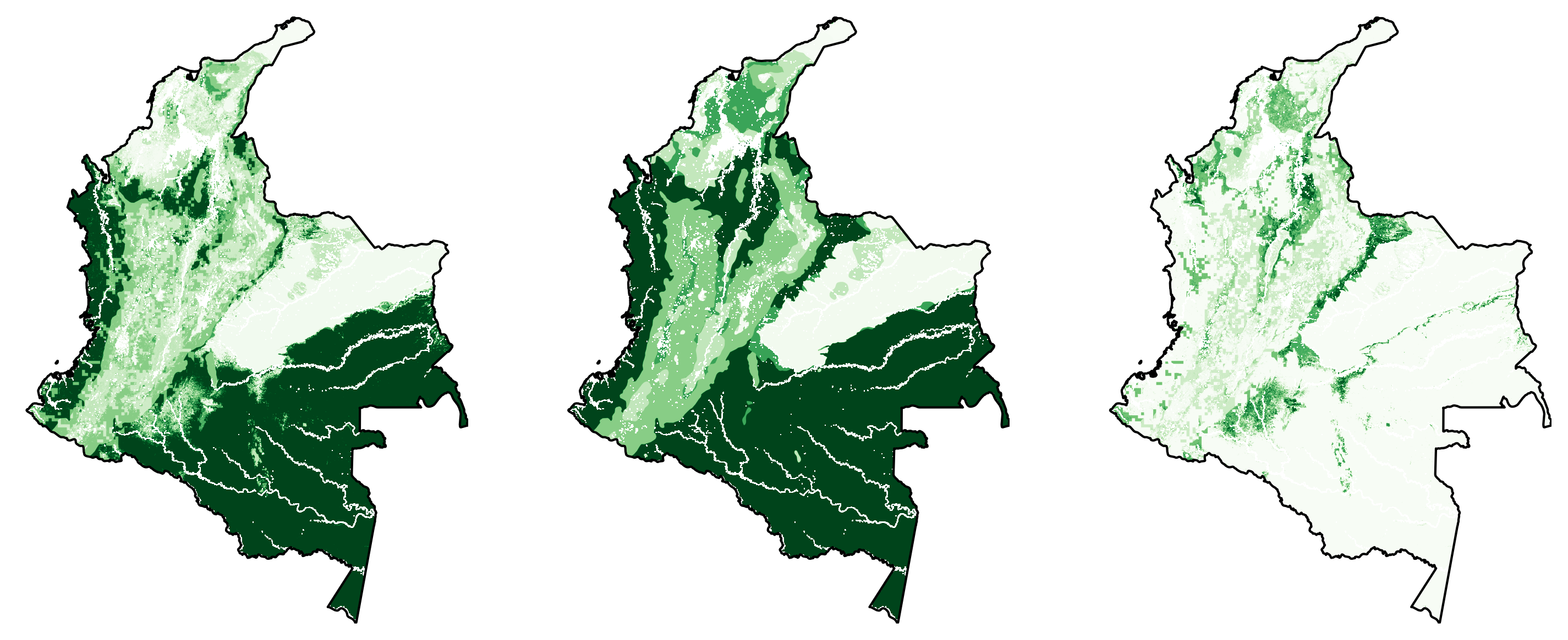
Panels show carbon storage in a) current landscape, b) restored landscape, and c) the gain in carbon storage with restoration (difference map).
Note: When preparing this data for ROOT, it is important that all rasters be provided with identical extent, projection, and pixel size. Additionally, there is a particular format for the csv tables used to tell ROOT which raster to use for which data value. These details are discussed in the interface guide.
Within ROOT, one key user-defined parameter is the “spatial decision unit” (SDU, see guide). This is the spatial unit for which ROOT turns each of the potential activities (in this case restoration) on or off. Due to computational limitations, it is generally not practical to have SDUs correspond with pixels. Depending on pixel size, this might also correspond with reasonable project limitations - for example it might not make sense to identify 30m^2 areas for restoration if there is a fixed per-project cost. Here we will set the SDUs to be 25 ha, but it is worth considering this choice carefully for any given application. Note that ROOT also allows the user to provide an explicit map (via a shapefile) of desired SDUs, giving a great deal of flexibility to how SDUs are structured.
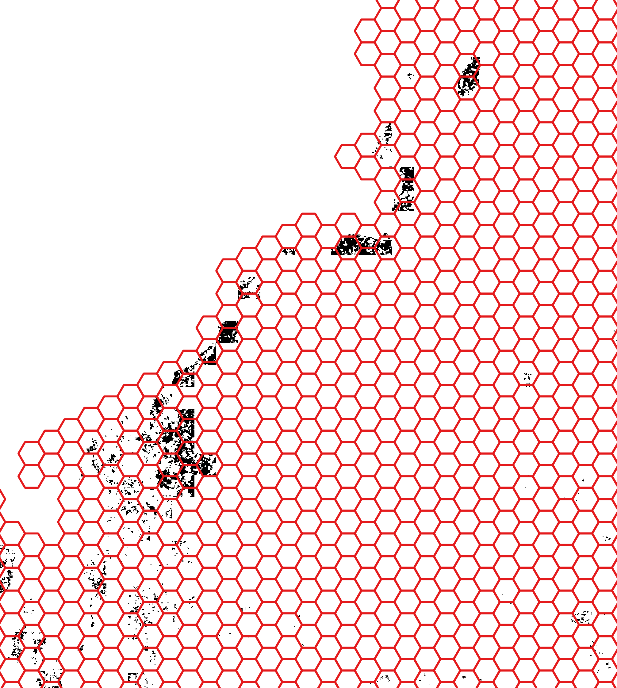
Example of hexagonal SDUs generated by ROOT preprocessing for this example.
With this data provided, we can run ROOT’s preprocessing step, which calculates per-SDU totals for each of the provided potential impact rasters. This step automates masking the impact rasters according to the activity and area-of-interest masks and performing the zonal stats needed to sum the impact per SDU polygon. The results are saved to tables of values used by the optimization step, as well as to a shapefile output that can be used for user analysis or visualization.
2.1.3. Optimization parameters
Finally, we need to specify the kind of optimization analysis to run. Within a ROOT optimization problem, there are three elements to consider: what are the choices available? What are the objectives or goals of the decision? And what are the constraints or targets? We have discussed the first of these already - the various activities available in each SDU are the choices. More specifically, the choices are to do or not do a given activity in each of the various SDUs.
The objectives define the values that we aim to maximize or minimize with different allocations of the various activities. In our current example the objectives are:
Improvement in a biodiversity index
Increase in carbon storage
Reduction in nitrate concentrations in drinking water
In this example, each of these has been calculated so that a larger value represents a bigger benefit, although ROOT can handle objectives where a smaller value is preferable as well (e.g. total nitrate rather than reduction of nitrate, or cost). When identifying each objective, the user must indicate whether to maximize or minimize it.
Constraints (targets) are rules that determine which allocations of the activities are valid. Some familiar constraints might be a total budget that can’t be exceeded, or a critical area of habitat that needs to be protected. In ROOT, constraints can be set on multiple elements at a time, allowing for some relatively complex problem formulations to be addressed. In this example, we will set a constraint on the total area to restore.
Note that it is possible to treat some value either as an objective or constraint (or both). For example, the user could set a budget constraint and examine the range of possible environmental benefits in one analysis, while in another set a fixed environmental goal and solve for the least-cost solution. In the optimization literature, these two approaches are called “dual problems” of each other.
Finally, we must specify what kind of analysis ROOT will perform. These options are explained in more detail in the guide, but for now, since we are interested in capturing the full range of the possible co-benefits to biodiversity, carbon, and water quality, we will use the “n dim frontier” option. The n-dimensional frontier choice will randomly sample from across the range of combinations of each given objective. For this analysis, we set the optimization to maximize each of the environmental objectives with a target value of 10,000 ha of the restoration activity. Note that almost all single-activity ROOT analyses will need a constraint of some kind. Without one, the optimization is likely to select all possible activity locations, which is unlikely to be useful information.
2.1.4. Running the analysis
After we get the data in place, the input files to ROOT configured, and the optimization parameters specified, we can click “Run”. (Note it is also possible to run the preprocessing and optimization steps separately, which we will see in a following example)
When it runs, the optimizer packaged with ROOT will solve a sequence of optimizations, each one of which generates a particular optimized allocation of 10,000 ha of restoration among the potential restoration sites we identified. The optimizations differ in how much they prioritize maximizing any objective over another. Formally, they maximize a weighted sum of the objectives, with random weights selected for each run to cover a wide range of combinations.
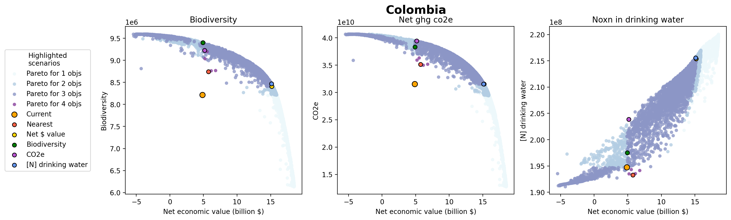
Optimization outputs showing frontiers for biodiversity, carbon, and water quality vs crop production value. Each dot represents the value of one optimization solution.
The output from the analysis is this set of specific solutions as well as an “agreement map” which identifies how often a particular SDU was selected for restoration among all solutions. SDUs that score highly in the agreement map are ones that are generally good choices regardless of the final preference between maximizing biodiversity, carbon, or water quality.
2.2. Extensions
The following examples expand on the base case to consider more complex applications of ROOT.
2.2.1. Multiple activities
In the first example, we considered a case where there was only one option being considered. In many cases we will want to consider allocation of multiple different activities, which could differ in where they could go and their impact across the objectives of interest. For example, we might want to consider restoration alongside protection and changes in agricultural production practices.
In these cases, we need to provide some additional data to ROOT. Similar to the first example, we need an activity mask and set of impact rasters for each of the activities. Additionally, we will need to apply some constraint either to each activity separately or to both activities together. An example of the former would be setting an area target for each activity individually, while an example of the latter would be setting a total budget for all activities together.
2.2.2. Adding in spatial weighting
Spatial weighting is a way of accounting for the fact that the same biophysical change may have a different social value depending on where it takes place. Some examples are changes in sediment loading upstream from a reservoir vs downstream of one, or reduction in NOx emissions upwind of a major population center vs reduction in a more remote area. Other reasons to include spatial weighting involve upweighting key areas of interest for biodiversity or using spatial weights to prioritize ecosystem benefits in areas of higher poverty.
Adding spatial weighting can be done pre-ROOT by “baking it in” to the impact rasters. For example, if the impact rasters are already in terms of a monetary damage (or benefit) that takes account of service flows, then no additional spatial weighting will be needed inside ROOT. On the other hand, if the impact raster is in terms of kg avoided sediment loss, a purely biophysical variable, then it might make sense to apply spatial weighting to help translate that into a social value variable.
Doing so in ROOT requires two steps. First, providing the spatial weighting map, which is a shapefile outlining regions to be differently weighted with a field assigning the weight scores to each region. ROOT will calculate the overlapping are of each weighting region with each SDU to calculate the relative weight factor to assign to each SDU. Second, using the combined factors tool to create weighted variables that combine a weighting factor with one (or more) of the impact scores.
NOTE: currently ROOT does not provide a method to apply spatial weighting via rasters. If you would like to use a raster to assign weights, please do this by multiplying the rasters with GIS software and then using this weighted output as an impact raster.
2.2.3. Absolute vs marginal values
In the example above, we used rasters that indicated the state of each objective under each of the potential landscape managements (baseline, restoration, etc…). This is the “absolute value” approach to a ROOT analsis. In other cases, it might make more sense to thing about the additional value that would be produced under some given change, also known as the “marginal value” of that change. In order to use ROOT in this way, simply omit the baseline scenario and provide value rasters measured in terms of the change from baseline to the alternative management.
2.2.4. Examples of optimization configurations
Here we provide some examples of objective and constraints that can be applied to investigate various problems:
Iterating through a range of area-based constraints and then overlaying the resulting frontiers in the same graph can be very helpful in picking the total target area. The same can be done with costs instead of area if there are costs associated with the activities.
Set the objective to minimize cost and set target (minimum) values for the environmental objectives. In this case, just run a single optimization to find the least-cost activity allocation that meets the environmental targets.
Consider including competing objectives. For example, by including crop production as an objective and also trying to maximize it, we can identify locations that provide the greatest environmental benefit relative to the lost agricultural production.
2.2.5. Spatial distributions
Let’s consider a case where we have target restoration areas, \(A_i\), for several different regions, but we want to optimize them simultaneously. Here are two ways to do that in ROOT:
Define restoration in each region as its own activity and provide distinct activity masks for each region. Then set constraints on the area in each region such as “region_name_ha” \(= A_i\).
Define spatial weighting masks for each region and create composite factors that combine the spatial extent and activity area to create a new variable. Set constraints on those new variables.
These approaches are identical from the perspective of the optimization tool, but hopefully give you some ideas of how to approach similar problems.
More examples to come